South American Indian vs Chickasaw Community Comparison
COMPARE
South American Indian
Chickasaw
Social Comparison
Social Comparison
South American Indians
Chickasaw
4,820
SOCIAL INDEX
45.7/ 100
SOCIAL RATING
193rd/ 347
SOCIAL RANK
3,663
SOCIAL INDEX
34.2/ 100
SOCIAL RATING
212th/ 347
SOCIAL RANK
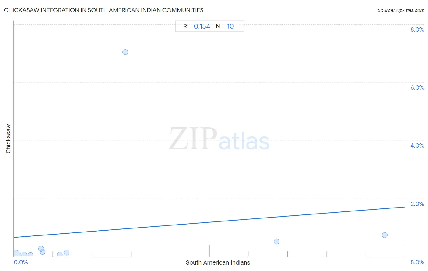
Chickasaw Integration in South American Indian Communities
The statistical analysis conducted on geographies consisting of 79,303,606 people shows a poor positive correlation between the proportion of Chickasaw within South American Indian communities in the United States with a correlation coefficient (R) of 0.154. On average, for every 1% (one percent) increase in South American Indians within a typical geography, there is an increase of 0.131% in Chickasaw. To illustrate, in a geography comprising of 100,000 individuals, a rise of 1,000 South American Indians corresponds to an increase of 131.3 Chickasaw.
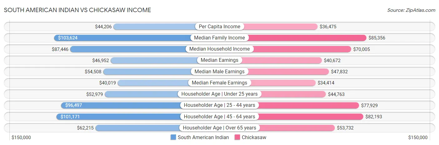
South American Indian vs Chickasaw Income
When considering income, the most significant differences between South American Indian and Chickasaw communities in the United States are seen in median household income ($87,446 compared to $70,005, a difference of 24.9%), householder income ages 25 - 44 years ($96,497 compared to $77,929, a difference of 23.8%), and householder income ages 45 - 64 years ($101,171 compared to $82,193, a difference of 23.1%). Conversely, both communities are more comparable in terms of wage/income gap (24.7% compared to 27.2%, a difference of 9.8%), median male earnings ($54,508 compared to $47,832, a difference of 14.0%), and median earnings ($46,952 compared to $40,672, a difference of 15.4%).
| Income Metric | South American Indian | Chickasaw |
| Per Capita Income | Good $44,206 | Tragic $36,475 |
| Median Family Income | Good $103,624 | Tragic $85,356 |
| Median Household Income | Excellent $87,446 | Tragic $70,005 |
| Median Earnings | Good $46,952 | Tragic $40,672 |
| Median Male Earnings | Average $54,508 | Tragic $47,832 |
| Median Female Earnings | Good $40,019 | Tragic $34,414 |
| Householder Age | Under 25 years | Excellent $52,979 | Tragic $44,763 |
| Householder Age | 25 - 44 years | Good $96,497 | Tragic $77,929 |
| Householder Age | 45 - 64 years | Good $101,171 | Tragic $82,193 |
| Householder Age | Over 65 years | Good $62,215 | Tragic $53,732 |
| Wage/Income Gap | Exceptional 24.7% | Tragic 27.2% |
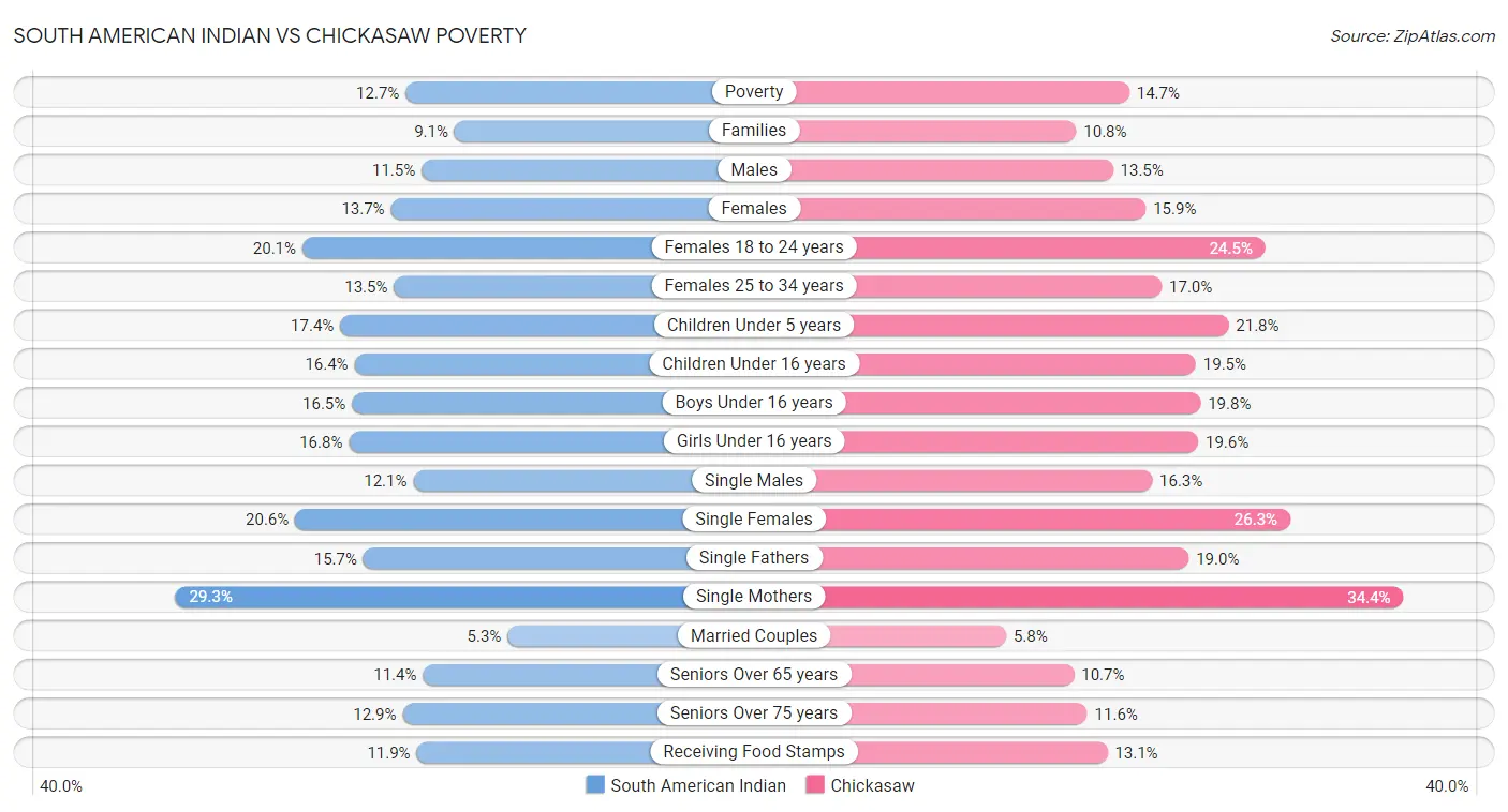
South American Indian vs Chickasaw Poverty
When considering poverty, the most significant differences between South American Indian and Chickasaw communities in the United States are seen in single male poverty (12.1% compared to 16.3%, a difference of 34.6%), single female poverty (20.6% compared to 26.3%, a difference of 27.3%), and female poverty among 25-34 year olds (13.5% compared to 17.0%, a difference of 25.9%). Conversely, both communities are more comparable in terms of seniors poverty over the age of 65 (11.4% compared to 10.7%, a difference of 6.9%), married-couple family poverty (5.3% compared to 5.8%, a difference of 8.6%), and receiving food stamps (11.9% compared to 13.1%, a difference of 10.3%).
| Poverty Metric | South American Indian | Chickasaw |
| Poverty | Fair 12.7% | Tragic 14.7% |
| Families | Fair 9.1% | Tragic 10.8% |
| Males | Fair 11.5% | Tragic 13.5% |
| Females | Fair 13.7% | Tragic 15.9% |
| Females 18 to 24 years | Average 20.1% | Tragic 24.5% |
| Females 25 to 34 years | Average 13.5% | Tragic 17.0% |
| Children Under 5 years | Average 17.4% | Tragic 21.8% |
| Children Under 16 years | Average 16.4% | Tragic 19.5% |
| Boys Under 16 years | Average 16.5% | Tragic 19.8% |
| Girls Under 16 years | Fair 16.8% | Tragic 19.6% |
| Single Males | Exceptional 12.1% | Tragic 16.3% |
| Single Females | Good 20.6% | Tragic 26.3% |
| Single Fathers | Exceptional 15.7% | Tragic 19.0% |
| Single Mothers | Average 29.3% | Tragic 34.4% |
| Married Couples | Fair 5.3% | Tragic 5.8% |
| Seniors Over 65 years | Poor 11.4% | Good 10.7% |
| Seniors Over 75 years | Tragic 12.9% | Exceptional 11.6% |
| Receiving Food Stamps | Average 11.9% | Tragic 13.1% |
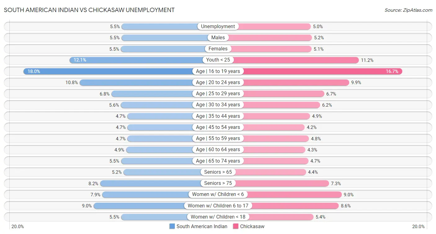
South American Indian vs Chickasaw Unemployment
When considering unemployment, the most significant differences between South American Indian and Chickasaw communities in the United States are seen in unemployment among seniors over 65 years (5.2% compared to 4.4%, a difference of 18.4%), unemployment among ages 65 to 74 years (5.5% compared to 4.7%, a difference of 17.4%), and unemployment among ages 60 to 64 years (4.9% compared to 4.3%, a difference of 13.1%). Conversely, both communities are more comparable in terms of unemployment among ages 25 to 29 years (6.8% compared to 6.7%, a difference of 0.42%), unemployment among ages 55 to 59 years (4.7% compared to 4.8%, a difference of 1.8%), and unemployment among women with children under 18 years (5.5% compared to 5.4%, a difference of 2.9%).
| Unemployment Metric | South American Indian | Chickasaw |
| Unemployment | Tragic 5.5% | Exceptional 5.0% |
| Males | Tragic 5.5% | Excellent 5.2% |
| Females | Tragic 5.5% | Excellent 5.1% |
| Youth < 25 | Tragic 12.1% | Exceptional 11.2% |
| Age | 16 to 19 years | Poor 18.0% | Exceptional 16.7% |
| Age | 20 to 24 years | Tragic 10.8% | Exceptional 9.9% |
| Age | 25 to 29 years | Fair 6.8% | Fair 6.7% |
| Age | 30 to 34 years | Fair 5.6% | Tragic 6.2% |
| Age | 35 to 44 years | Average 4.7% | Tragic 4.9% |
| Age | 45 to 54 years | Tragic 4.7% | Exceptional 4.2% |
| Age | 55 to 59 years | Exceptional 4.7% | Good 4.8% |
| Age | 60 to 64 years | Fair 4.9% | Exceptional 4.3% |
| Age | 65 to 74 years | Tragic 5.5% | Exceptional 4.7% |
| Seniors > 65 | Poor 5.2% | Exceptional 4.4% |
| Seniors > 75 | Exceptional 8.2% | Exceptional 7.3% |
| Women w/ Children < 6 | Tragic 7.9% | Tragic 9.0% |
| Women w/ Children 6 to 17 | Fair 9.0% | Exceptional 8.6% |
| Women w/ Children < 18 | Fair 5.5% | Good 5.4% |
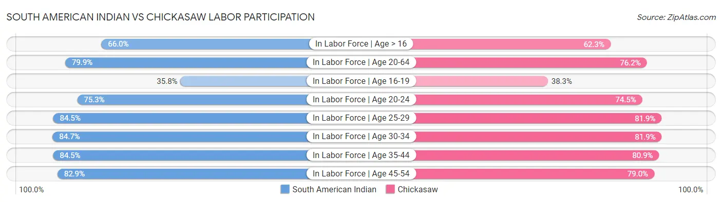
South American Indian vs Chickasaw Labor Participation
When considering labor participation, the most significant differences between South American Indian and Chickasaw communities in the United States are seen in in labor force | age 16-19 (35.8% compared to 38.3%, a difference of 7.2%), in labor force | age > 16 (66.0% compared to 62.3%, a difference of 6.0%), and in labor force | age 20-64 (79.9% compared to 76.2%, a difference of 4.8%). Conversely, both communities are more comparable in terms of in labor force | age 20-24 (75.3% compared to 74.5%, a difference of 1.1%), in labor force | age 25-29 (84.5% compared to 81.9%, a difference of 3.2%), and in labor force | age 30-34 (84.7% compared to 81.9%, a difference of 3.4%).
| Labor Participation Metric | South American Indian | Chickasaw |
| In Labor Force | Age > 16 | Exceptional 66.0% | Tragic 62.3% |
| In Labor Force | Age 20-64 | Excellent 79.9% | Tragic 76.2% |
| In Labor Force | Age 16-19 | Poor 35.8% | Exceptional 38.3% |
| In Labor Force | Age 20-24 | Good 75.3% | Poor 74.5% |
| In Labor Force | Age 25-29 | Fair 84.5% | Tragic 81.9% |
| In Labor Force | Age 30-34 | Average 84.7% | Tragic 81.9% |
| In Labor Force | Age 35-44 | Good 84.5% | Tragic 80.9% |
| In Labor Force | Age 45-54 | Good 82.9% | Tragic 79.0% |
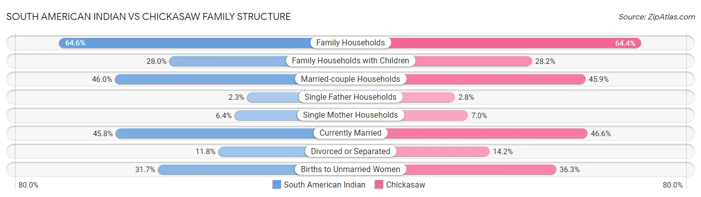
South American Indian vs Chickasaw Family Structure
When considering family structure, the most significant differences between South American Indian and Chickasaw communities in the United States are seen in single father households (2.3% compared to 2.8%, a difference of 22.3%), divorced or separated (11.8% compared to 14.2%, a difference of 20.4%), and births to unmarried women (31.7% compared to 36.3%, a difference of 14.3%). Conversely, both communities are more comparable in terms of married-couple households (46.0% compared to 45.9%, a difference of 0.28%), family households (64.6% compared to 64.4%, a difference of 0.35%), and family households with children (28.0% compared to 28.2%, a difference of 0.91%).
| Family Structure Metric | South American Indian | Chickasaw |
| Family Households | Excellent 64.6% | Good 64.4% |
| Family Households with Children | Exceptional 28.0% | Exceptional 28.2% |
| Married-couple Households | Fair 46.0% | Fair 45.9% |
| Average Family Size | Exceptional 3.26 | Tragic 3.19 |
| Single Father Households | Excellent 2.3% | Tragic 2.8% |
| Single Mother Households | Fair 6.4% | Tragic 7.0% |
| Currently Married | Poor 45.8% | Average 46.6% |
| Divorced or Separated | Exceptional 11.8% | Tragic 14.2% |
| Births to Unmarried Women | Average 31.7% | Tragic 36.3% |
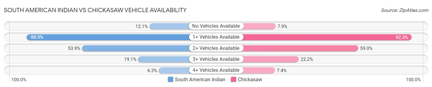
South American Indian vs Chickasaw Vehicle Availability
When considering vehicle availability, the most significant differences between South American Indian and Chickasaw communities in the United States are seen in no vehicles in household (12.1% compared to 7.9%, a difference of 53.5%), 4 or more vehicles in household (6.3% compared to 7.4%, a difference of 18.7%), and 3 or more vehicles in household (19.1% compared to 22.2%, a difference of 16.2%). Conversely, both communities are more comparable in terms of 1 or more vehicles in household (88.0% compared to 92.3%, a difference of 4.8%), 2 or more vehicles in household (53.9% compared to 59.0%, a difference of 9.5%), and 3 or more vehicles in household (19.1% compared to 22.2%, a difference of 16.2%).
| Vehicle Availability Metric | South American Indian | Chickasaw |
| No Vehicles Available | Tragic 12.1% | Exceptional 7.9% |
| 1+ Vehicles Available | Tragic 88.0% | Exceptional 92.3% |
| 2+ Vehicles Available | Tragic 53.9% | Exceptional 59.0% |
| 3+ Vehicles Available | Fair 19.1% | Exceptional 22.2% |
| 4+ Vehicles Available | Average 6.3% | Exceptional 7.4% |
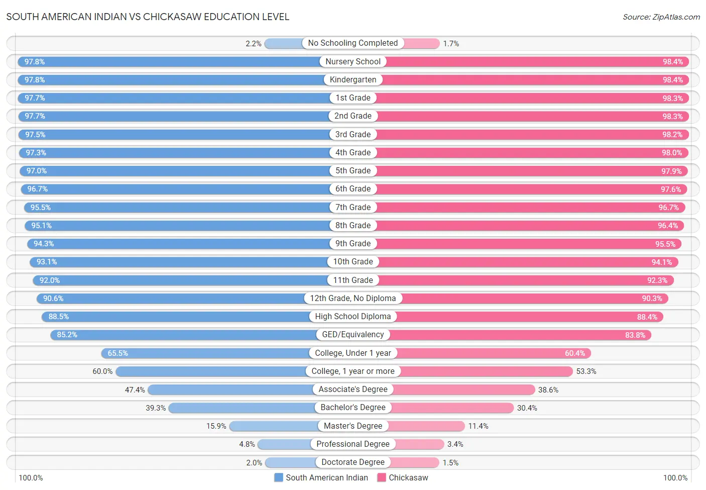
South American Indian vs Chickasaw Education Level
When considering education level, the most significant differences between South American Indian and Chickasaw communities in the United States are seen in professional degree (4.8% compared to 3.4%, a difference of 41.5%), master's degree (15.9% compared to 11.4%, a difference of 39.1%), and no schooling completed (2.2% compared to 1.7%, a difference of 32.1%). Conversely, both communities are more comparable in terms of high school diploma (88.5% compared to 88.4%, a difference of 0.060%), 12th grade, no diploma (90.6% compared to 90.3%, a difference of 0.28%), and 11th grade (92.0% compared to 92.3%, a difference of 0.42%).
| Education Level Metric | South American Indian | Chickasaw |
| No Schooling Completed | Poor 2.2% | Exceptional 1.7% |
| Nursery School | Tragic 97.8% | Exceptional 98.4% |
| Kindergarten | Tragic 97.8% | Exceptional 98.4% |
| 1st Grade | Tragic 97.7% | Exceptional 98.3% |
| 2nd Grade | Tragic 97.7% | Exceptional 98.3% |
| 3rd Grade | Tragic 97.5% | Exceptional 98.2% |
| 4th Grade | Tragic 97.3% | Exceptional 98.0% |
| 5th Grade | Tragic 97.0% | Exceptional 97.9% |
| 6th Grade | Tragic 96.7% | Exceptional 97.6% |
| 7th Grade | Tragic 95.5% | Exceptional 96.7% |
| 8th Grade | Tragic 95.1% | Exceptional 96.4% |
| 9th Grade | Tragic 94.3% | Exceptional 95.5% |
| 10th Grade | Tragic 93.1% | Excellent 94.1% |
| 11th Grade | Tragic 92.0% | Fair 92.3% |
| 12th Grade, No Diploma | Poor 90.6% | Tragic 90.3% |
| High School Diploma | Poor 88.5% | Poor 88.4% |
| GED/Equivalency | Fair 85.2% | Tragic 83.8% |
| College, Under 1 year | Average 65.5% | Tragic 60.4% |
| College, 1 year or more | Good 60.0% | Tragic 53.3% |
| Associate's Degree | Good 47.4% | Tragic 38.6% |
| Bachelor's Degree | Excellent 39.3% | Tragic 30.4% |
| Master's Degree | Excellent 15.9% | Tragic 11.4% |
| Professional Degree | Excellent 4.8% | Tragic 3.4% |
| Doctorate Degree | Excellent 2.0% | Tragic 1.5% |
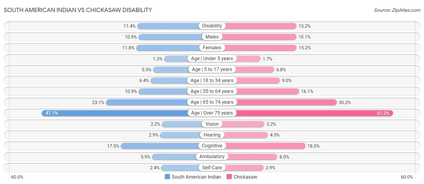
South American Indian vs Chickasaw Disability
When considering disability, the most significant differences between South American Indian and Chickasaw communities in the United States are seen in hearing disability (2.9% compared to 4.5%, a difference of 56.4%), disability age 35 to 64 (10.9% compared to 16.1%, a difference of 47.7%), and vision disability (2.2% compared to 3.2%, a difference of 47.4%). Conversely, both communities are more comparable in terms of cognitive disability (17.5% compared to 18.5%, a difference of 5.6%), disability age over 75 (47.1% compared to 51.2%, a difference of 8.6%), and self-care disability (2.4% compared to 2.9%, a difference of 18.6%).
| Disability Metric | South American Indian | Chickasaw |
| Disability | Exceptional 11.4% | Tragic 15.2% |
| Males | Excellent 10.9% | Tragic 15.1% |
| Females | Exceptional 11.8% | Tragic 15.2% |
| Age | Under 5 years | Tragic 1.3% | Tragic 1.7% |
| Age | 5 to 17 years | Excellent 5.5% | Tragic 6.8% |
| Age | 18 to 34 years | Excellent 6.4% | Tragic 9.0% |
| Age | 35 to 64 years | Excellent 10.9% | Tragic 16.1% |
| Age | 65 to 74 years | Good 23.1% | Tragic 30.2% |
| Age | Over 75 years | Good 47.1% | Tragic 51.2% |
| Vision | Average 2.2% | Tragic 3.2% |
| Hearing | Excellent 2.9% | Tragic 4.5% |
| Cognitive | Poor 17.5% | Tragic 18.5% |
| Ambulatory | Exceptional 5.9% | Tragic 8.0% |
| Self-Care | Excellent 2.4% | Tragic 2.9% |